Training the Predictor: From Data to Decision-Ready Models

Today we will finally jump into the fun part, the part where we actually train our machine learning models: the training pipeline.

Welcome back to the CAI deep-dive series. If you’ve followed our previous newsletters, you’ve seen how we bridge the gap between installation and orchestration, walked through the ingestion pipeline that transforms 1,000+ trades per second into ML-ready features, and tackled the orchestration layer that keeps production systems breathing.

Now we’re stepping into the training pipeline, the stage where features become a model, where hypotheses are tested, and where we answer the million-dollar question: can our machine learning model actually predict market movements?

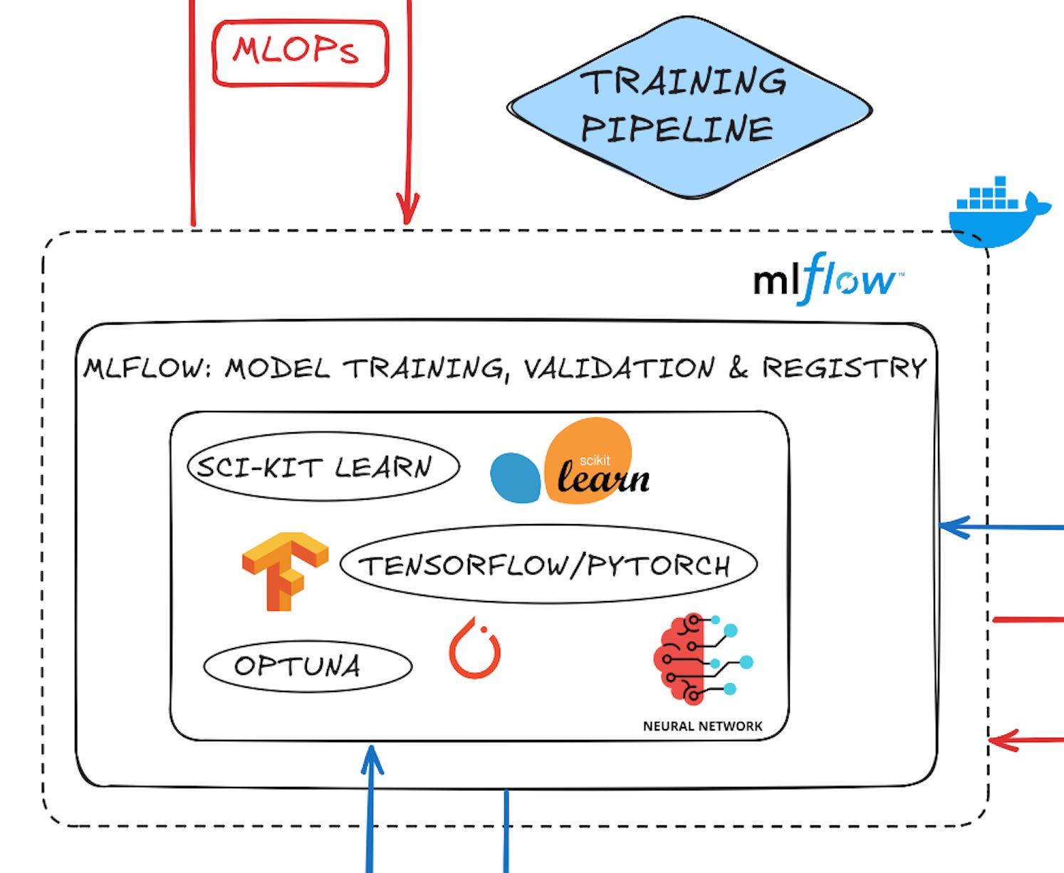
The training pipeline sits at the heart of CAI. It’s where the orchestrator sends clean, engineered data, and where MLflow, Optuna together with our modelling framework of choice - scikit-learn, TensorFlow, or PyTorch - converge into a systematic hyperparameter optimization and model validation framework.

Unlike traditional ML tutorials that treat training as a black box (”just call .fit() and hope”), we’re building something intentional. Every decision is tracked. Every trial is logged. Every failure teaches us something quantifiable.

Why the Training Pipeline Matters

Here’s what most ML tutorials won’t tell you: the model isn’t the hard part. The hard part is knowing which model to build, how to build it reproducibly, and why it works when it does.

In production systems, this distinction is critical. Three months from now, your model will drift. A competitor’s data source will disappear. The market regime will shift. When that happens, you won’t just retrain: you’ll need to understand what changed, compare it to previous training runs, and make an evidence-based decision about whether to rollback, iterate, or start over.

That’s where the training pipeline becomes infrastructure. It’s not just about fitting models. It’s about creating an auditable record of every experiment, every hyperparameter sweep, and every decision that led to your current production model.

The Architecture: Four Connected Boxes

Let me introduce the flow (and yes, if you’ve been following our series, you know we’re obsessed with systems thinking. Everything is boxes that talk to each other):

Raw Data → [Training Pipeline] → Model Registry → [Prediction API]
               ↓
         ┌─────┴─────────────────────┐
         ↓                           ↓
    [Feature Engineering]    [Hyperparameter Optimization]
         ↓                           ↓
    [Data Splitting]         [Trial Execution]
         ↓                           ↓
    [Model Training]         [Metric Logging]
    (PyTorch, TensorFlow,         (MLflow)
      scikit-learn)
         ↓
    [Validation & Testing]
         ↓
    [Model Versioning]
         ↓
    MLflow Registry

---

The training pipeline in CAI orchestrates three key layers (and we will add the data engineering layer before the other 3 for the sake of completeness):

1. Data Layer: Feature engineering and train/test splits

2. Optimization Layer: Optuna searching the hyperparameter space

3. Training Layer: PyTorch/TensorFlow/scikit-learn executing the actual training

4. Tracking Layer: MLflow logging every parameter, metric, and artifact

Let’s walk through each.

Layer 1: Data Preparation. The Foundation Everything Rests On

If you’ve been following along you know already what happens here, but a little refresher won’t harm anyone. After all, data pre-processing is the foundation that determines whether your entire experiment is meaningful or noise.

In CAI’s predictor service, we receive engineered features from the ingestion pipelin: technical indicators, OHLCV candles, volume profiles. But raw features aren’t ready for training. We need to:

Normalize and scale: ML models - and Neural networks especially - are sensitive to feature magnitude. We use standardization (mean-centering and scaling by standard deviation) so a feature ranging 0-1 doesn’t dwarf a feature ranging 0-100. This is especially critical when we mix momentum indicators (RSI: 0-100), moving averages (absolute price), and volatility measures (standard deviation).

Handle temporal structure: Crypto prices are time series data. We can’t randomly shuffle our training set, as this breaks the temporal dependencies. Instead, we split chronologically: train on data from January-September, validate on October-November, test on December. This mimics how your model will actually operate: making predictions on data it has never seen, but in a time-sequential manner.

Create sequences: For advanced ML models like LSTM or transformer-based architectures, we batch trades and features into sequences. A 60-minute window of candles becomes a single training example. The network learns patterns within that window and predicts the next candle’s movement.

In code, this looks conceptually like:

# Pseudocode for temporal data splitting
train_data = df[df[’timestamp’] < ‘2024-10-01’]
val_data = df[(df[’timestamp’] >= ‘2024-10-01’) & (df[’timestamp’] < ‘2024-11-01’)]
test_data = df[df[’timestamp’] >= ‘2024-11-01’]

# Normalize using training statistics only
scaler = StandardScaler()
scaler.fit(train_data)  # Fit on training data only
X_train = scaler.transform(train_data)
X_val = scaler.transform(val_data)
X_test = scaler.transform(test_data)

---

Notice the critical detail: the scaler is fit only on training data. If you normalize using test data statistics, you’re leaking information from your future into your past. Data leakage is how you end up with a model that looks brilliant in the lab but hemorrhages money in production.

Layer 2: Hyperparameter Optimization. The Thousand-Trial Search

Now we reach the part that distinguishes serious ML engineering from script-kidding: systematic hyperparameter optimization.

A ML model isn’t just its architecture. When developing artificial neural networks, every parameter that won’t get automatically updated by the backpropagation algorithm, is called a hyperparameter. It’s the learning rate, dropout rate, batch size, number of layers, activation functions, regularization coefficients, and a dozen other knobs.

In other words, every variable that you can tune/change only after running an experiment based on heuristics, experience or knowledge. This applies also for other algorithms besides artificial neural networks.

Manually tweaking these is like navigating New York City with a broken compass. You might find your way, but you’ll waste a lot of time and energy.

Optuna solves this by treating hyperparameter search as a structured optimization problem. Instead of random guessing, it uses algorithms (like TPE, a.k.a Tree-structured Parzen Estimator) that learn from previous trials and intelligently suggest new configurations to test. You could also use Bayesian Optimization or any other algorithm that you like. ML is also a little bit of alchemy sometimes.

Here’s how it works in practice:

import optuna
from optuna.integration.mlflow import MLflowCallback
import mlflow

def objective(trial):
    “”“Define a single training trial”“”
    
    # Suggest hyperparameters
    learning_rate = trial.suggest_loguniform(’learning_rate’, 1e-5, 1e-2)
    batch_size = trial.suggest_categorical(’batch_size’, [32, 64, 128])
    dropout_rate = trial.suggest_uniform(’dropout_rate’, 0.2, 0.7)
    num_layers = trial.suggest_int(’num_layers’, 2, 5)
    
    with mlflow.start_run(nested=True):
        # Log parameters
        mlflow.log_params({
            ‘learning_rate’: learning_rate,
            ‘batch_size’: batch_size,
            ‘dropout_rate’: dropout_rate,
            ‘num_layers’: num_layers
        })
        
        # Build and train model
        model = build_neural_network(
            num_layers=num_layers,
            dropout_rate=dropout_rate
        )
        optimizer = torch.optim.Adam(model.parameters(), lr=learning_rate)
        
        # Training loop
        for epoch in range(num_epochs):
            train_loss = train_epoch(model, train_loader, optimizer)
            val_loss = validate_epoch(model, val_loader)
            
            # Log metrics
            mlflow.log_metric(’train_loss’, train_loss, step=epoch)
            mlflow.log_metric(’val_loss’, val_loss, step=epoch)
            
            # Report intermediate value to Optuna for pruning
            trial.report(val_loss, epoch)
            
            # Prune trials that are clearly underperforming
            if trial.should_prune():
                raise optuna.TrialPruned()
        
        return val_loss

# Run the optimization
mlflc = MLflowCallback(tracking_uri=’mlruns’, metric_name=’val_loss’)
study = optuna.create_study(direction=’minimize’)
study.optimize(objective, n_trials=100, callbacks=[mlflc])

---

Notice three critical details:

Pruning: Optuna doesn’t run every trial to completion. If it’s clear after 10 epochs that this learning rate is rubbish, it kills the trial and moves on. This saves enormous computation time.

Nested MLflow runs: Each Optuna trial creates a nested MLflow run. The parent run aggregates 100 child runs. When you open MLflow’s UI later, you can see the entire hyperparameter search landscape: which hyperparameters correlated with good performance, which were red herrings.

Systematic searching: Unlike random search, Optuna learns. Early trials explore the space broadly. Later trials concentrate on promising regions. This is Bayesian optimization in practice balancing exploration and exploitation.

Layer 3: Training Layer. Where Neurons Learn

This is where PyTorch, TensorFlow, or scikit-learn actually execute. The model architecture depends on your problem. For crypto price prediction, recurrent networks (LSTMs, GRUs) or transformers often outperform feedforward networks because they capture temporal dependencies. If you look into our CAI repo we chose simpler algorithms after running our Optuna optimization, like the Huber Regression.

Here’s a minimal transformer-based architecture for price prediction:

import torch
import torch.nn as nn

class CryptoPricePredictionTransformer(nn.Module):
    def __init__(self, input_size, num_heads=4, num_layers=2, dropout=0.2):
        super().__init__()
        
        # Embedding layer (project raw features into hidden space)
        self.embedding = nn.Linear(input_size, 64)
        
        # Transformer encoder
        encoder_layer = nn.TransformerEncoderLayer(
            d_model=64,
            nhead=num_heads,
            dropout=dropout,
            batch_first=True
        )
        self.transformer = nn.TransformerEncoder(encoder_layer, num_layers=num_layers)
        
        # Prediction head
        self.fc = nn.Sequential(
            nn.Linear(64, 32),
            nn.ReLU(),
            nn.Dropout(dropout),
            nn.Linear(32, 1)  # Predict next price movement
        )
    
    def forward(self, x):
        # x shape: (batch_size, seq_length, input_size)
        x = self.embedding(x)  # -> (batch_size, seq_length, 64)
        x = self.transformer(x)  # -> (batch_size, seq_length, 64)
        x = x[:, -1, :]  # Take last timestep -> (batch_size, 64)
        return self.fc(x)

# Training loop (simplified)
model = CryptoPricePredictionTransformer(input_size=num_features)
optimizer = torch.optim.Adam(model.parameters(), lr=learning_rate)
criterion = nn.MSELoss()

for epoch in range(num_epochs):
    model.train()
    for X_batch, y_batch in train_loader:
        predictions = model(X_batch)
        loss = criterion(predictions, y_batch)
        
        optimizer.zero_grad()
        loss.backward()
        optimizer.step()
    
    # Validation
    model.eval()
    with torch.no_grad():
        val_loss = evaluate_on_validation_set(model, val_loader)

---

The architecture balances three goals: learning temporal patterns (transformers excel here), regularization (dropout prevents overfitting), and interpretability (we need to understand why the model made a prediction).

Layer 4: MLflow. Your Experiment Laboratory

Here’s where it gets powerful. MLflow is your lab notebook. Every model you train, every parameter you set, every metric you compute gets recorded.

When you navigate to mlflow ui and open your browser to localhost:5000, you see:

• Experiment tracking: Every trial grouped under a parent experiment. Compare runs side-by-side.

• Parameter logging: Which learning rates, batch sizes, and architectures led to the best performance?

• Metric tracking: Validation loss, training loss, accuracy. Whatever you log, you can graph and compare.

• Model versioning: Save the best model and tag it. Months later, you can trace back exactly which experiment produced your production model.

• Artifacts: Store feature engineering code, scaler objects, or even visualizations of the attention weights.

In production, this becomes critical. When your model starts drifting, you can ask: “What was different about the training run three months ago that worked better?” Then you reload that scaler, retrain with similar hyperparameters, and deploy the new version.

Closing the Loop: From Optuna to MLflow to Registry

The final step is the model registry. The best model from our 100 Optuna trials goes into MLflow’s registry with a tag: crypto_predictor_champion. From there, the predictor service knows exactly which model to load and how to preprocess data to match.

This is where systems thinking matters. The training pipeline doesn’t live in isolation. It connects to the ingestion pipeline (which sends features), the orchestration layer (which schedules retraining), and the prediction API (which consumes the model).

Why This Matters for Production ML

Most ML tutorials show you how to train a model on your laptop. They stop there. Real ML engineering answers harder questions:

• How do you systematically explore hyperparameter space without wasting compute?

• How do you reproduce a training run three months later?

• How do you know when retraining is necessary?

• How do you A/B test two models in production?

The training pipeline we’ve built here answers all of those. It’s not just elegant. It’s necessary.

Next Steps

In the next newsletter, we’ll zoom back out and talk about the prediction API layer: how this trained model actually serves real-time predictions, why latency matters more than you think, and how we monitor for model drift in production.

Until then, clone the CAI repo, spin up the predictor service, and watch Optuna search the hyperparameter space. There’s nothing quite like seeing 100 trials run in parallel and watching the best validation loss improve trial after trial.